解析频域和时域的关系

本文是德科技解析了关于频域和时域的关系。

频域和时域分析是分析信号的基本方法，是从不同的角度来描述信号的特性。信号的特性可以在时域上和频率域上得到反映。

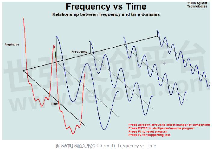
频域和时域的关系(Gif format）Frequency vs Time

信号的基本分析方法

谈到频域和时域关系，我们先从信号的基本分析方法讲起。传统上对无线、有线通讯信号的分析方法从三个域上划分：时域、频域和调制域。调制域是分析信号频率（或相位）随时间的变化。

频域和时域以及幅度的关系

频域测量

宽频率范围信号搜索
信号杂散测试
信号功率参数
信号占用频率带宽

时域测量

信号变化过程

解调测量

信号调制参数
信号调制精度

解调测量是对调制信号的幅相及频率变化进行测量的一种手段，是从另一个角度分析信号，和传统的三个域（及对应的示波器、频谱仪和调制域分析仪）有所不同，解调测量的概念对应的是矢量信号分析仪。

频域和时域的关系

时域(Time domain) ：分析信号参数随时间变化过程。时域是信号在时间轴随时间变化的总体概括。在时域中，将信号的所有频率分量相加并显示。频谱分析仪针对频域。

频域(Frequency domain)：分析信号包含的频率成分。各频率分量的频率和功率参数。在频域中，复数信号（即，由一个以上频率组成的信号）被分离成它们的频率分量，并显示每个频率的电平。示波器用来看时域内容。

因为信号不仅随时间变化，还与频率、相位等信息有关，这就需要进一步分析信号的频率结构，并在频率域中对信号进行描述。动态信号从时间域变换到频率域主要通过傅立叶级数和傅立叶变换等来实现。

时域函数通过傅立叶或者拉普拉斯变换就变成了频域函数

很简单时域分析的函数是参数是t，也就是y=f(t)，频域分析时，参数是w，也就是y=F(w)两者之间可以互相转化。时域函数通过傅立叶或者拉普拉斯变换就变成了频域函数。

频域和时域分析变换

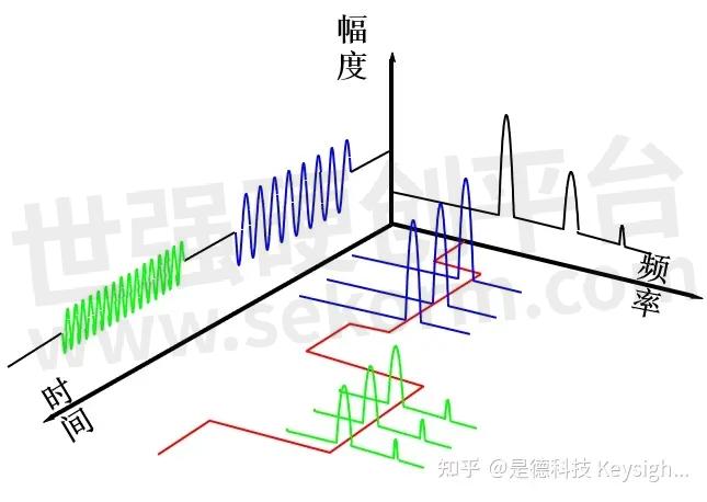
频域图1

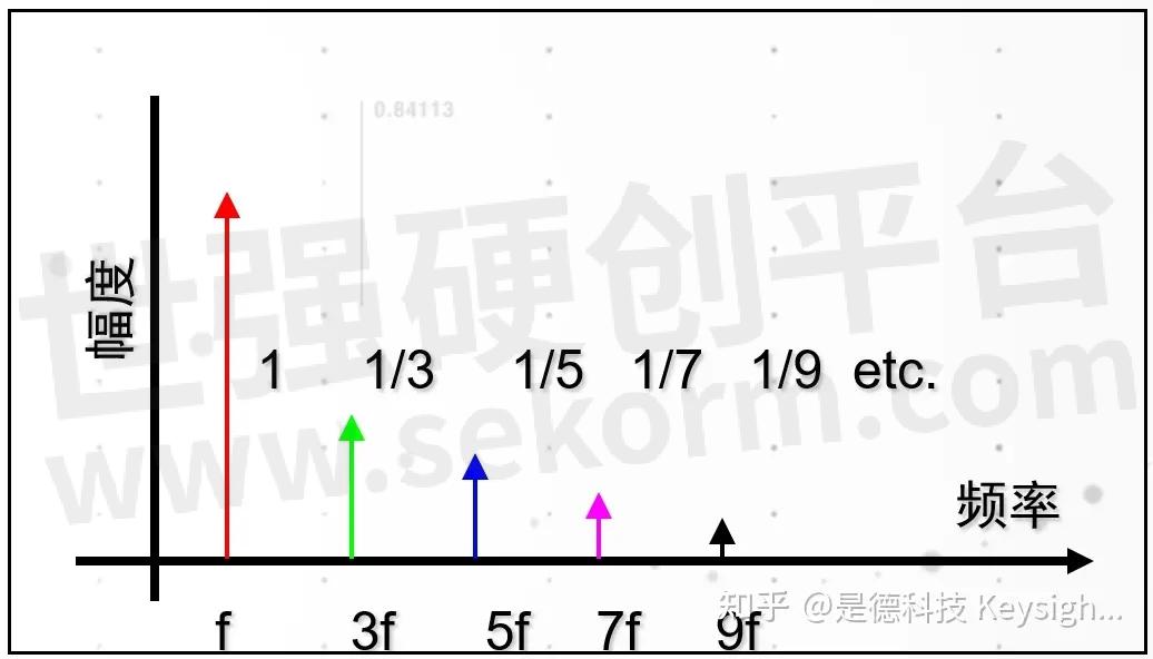
时域图1

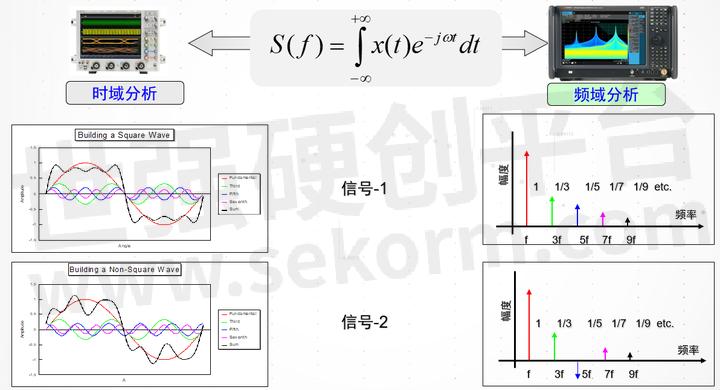
信号-1

频域图2

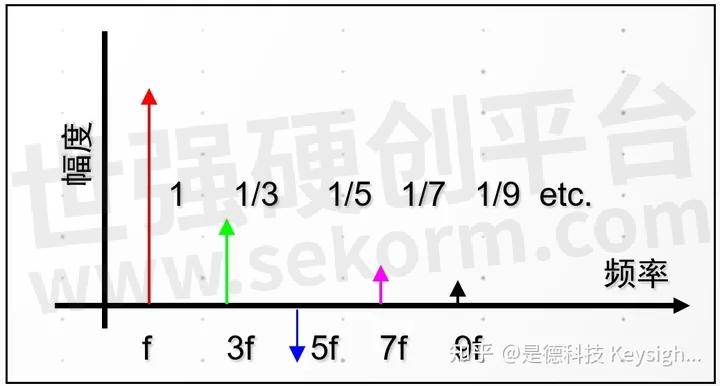
时域图2

信号-2

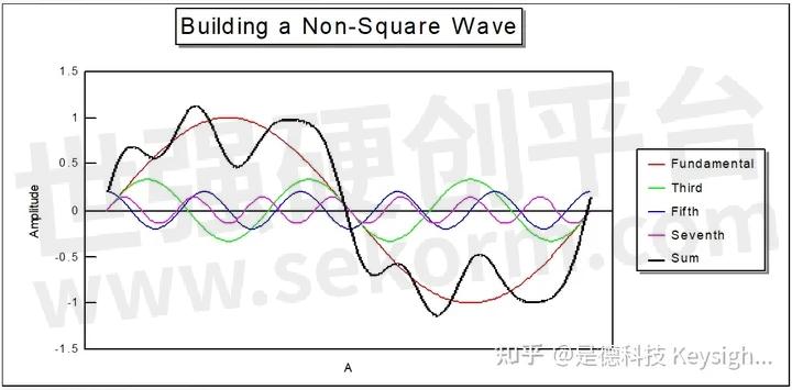
为什么要频域分析信号？（方波的例子）

作为常见信号分析的方法，可使用示波器测量信号时域波形。时域分析可直观反映信号幅度；频率；相位的变化。上图中时域的测试可以明显地观测到信号1和信号2时域波形（黑色轨迹）的区别。但只通过时域的观测很难判断两个信号波形差别的原因。

什么是频域分析？

所谓频域分析，就是在频率的坐标下分析信号。完整的频域分析应该得到被测信号包含的频率成分，还有每个频率成分的幅度和相位关系。即信号功率谱和相位谱的分析。某个信号的波形发生变化，其频谱特性会发生相应变化。频域和时域分析是分析信号的基本方法，是从不同的角度来描述信号的特性。

频域分析包括：
•分析信号的频率成分。各频率分量的频率与功率参数。
•信号功率，信号带宽，带外杂散，ACPR。

时域反射测量技术 (TDR) 和时域分析的历史

时域反射测量技术 (Time domain reflectometry (TDR)) 是在20世纪60年代初引入的，采用与雷达相同的工作原理 — 把一个冲激信号送入一条被测电缆 (或其他可能不是良好导体的被测器件或设备)，当该冲激信号到达电缆末端或电缆上的某个故障点时，一部分或全部冲激信号便会被返射回测试仪表。TDR 测量方法就是把一个冲激或阶跃激励信号发送到被测器件，然后观察信号在时域内的响应。测试时，使用一台阶跃信号发生器和一台宽带示波器，把阶跃信号发生器产生的上升沿速度极快的激励信号送进被测传输线，然后用宽带示波器观察传输线上某处入射电压波形和反射电压波形，通过测量入射电压与反射电压之比，便能计算出传输线上这个阻抗不连续点处的阻抗值，而这个阻抗不连续点的位置则可以作为时间函数根据信号沿着传输线传播的速度计算出来。阻抗不连续性的性质(电容性的或电感性的) 可以根据其信号的响应特征加以识别。

虽然我们过去惯用的TDR示波器作为定性测试工具一直非常有用，但存在一些影响其测试精度和有效性的限制因素: a) TDR输出的阶跃信号的上升时间—测量结果在空间上的分辨率取决于阶跃信号上升时间的快慢；b) 不是特别理想的信噪比－这是由于示波器宽带接收机的结构引起的。

随后，在70年代，研究表明频域与时域之间的关系可以用傅立叶变换进行描述。

与频率有关的网络反射系数经过傅立叶变换之后就可以得到随时间变化的反射系数，例如传输线上的距离。这样就有可能先在频域内测量被测器件的响应，然后用数学方法对这些频域数据进行傅立叶逆变换计算从而给出时域响应。

现在，一台高性能的矢量网络分析仪可以具有极快的计算功能，因而衍生出一些独特的测量能力。使用在频域内误差经过校正的测试数据就可以计算出被测网络对阶跃或冲激激励信号的响应，并且显示为时间函数。这样就给传统的时域反射测量技术提供了既能进行传输测试又能进行反射测试的功能，并增添了对带宽有限制的网络的测量能力。矢量网络分析仪在时域的测试可以更为精密，因为它能找出多余的网络部件的位置，从而把这些不需要的数据从被测数据去除掉。

下图显示的是无论是使用时域反射计 (TDR) 示波器还是使用矢量网络分析仪 (VNA) 都可以得到时域和频域 (S参数) 的显示结果，使用TDR或VNA得到的测试结果可以在两种显示形式中互相转换。

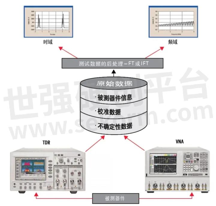
图  频域和时域、TDR和VNA之间的关系。

傅立叶变换

Here is a brief review of Fourier theory, especially the unique behaviour of the FFT. The note also describes some typical applications and provides some tips on how to get the most out of the FFT capability of the KEYSIGHT oscilloscopes.

Equipment Required

Keysight Oscilloscope-with FFT option (Note: units operate differently in some cases.)

Fourier Theory

Normally, when a signal is measured with an oscilloscope, it is viewed in the time domain (Figure 1a). That is, the vertical axis is voltage and the horizontal axis is time. For many signals, this is the most logical and intuitive way to view them. But when the frequency content of the signal is of interest, it makes sense to view the signal in the frequency domain. In the frequency domain, the vertical axis is still voltage but the horizontal axis is frequency (Figure 1b). The frequency domain display shows how much of the signal's energy is present at each frequency. For a simple signal such as a sine wave, the frequency domain representation does not usually show us much additional information. However, with more complex signals, the frequency content is difficult to uncover in the time domain and the frequency domain gives a more useful view of the signal.

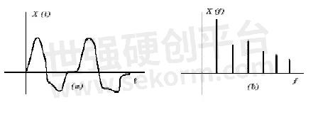
Figure1

(a) A signal shown as a function of time.

(b) A signal shown as a function of frequency.

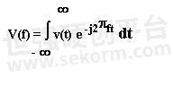
Fourier theory (including both the Fourier Series and the Fourier Transform) mathematically relates the time domain and the frequency domain. The Fourier transform is given by:

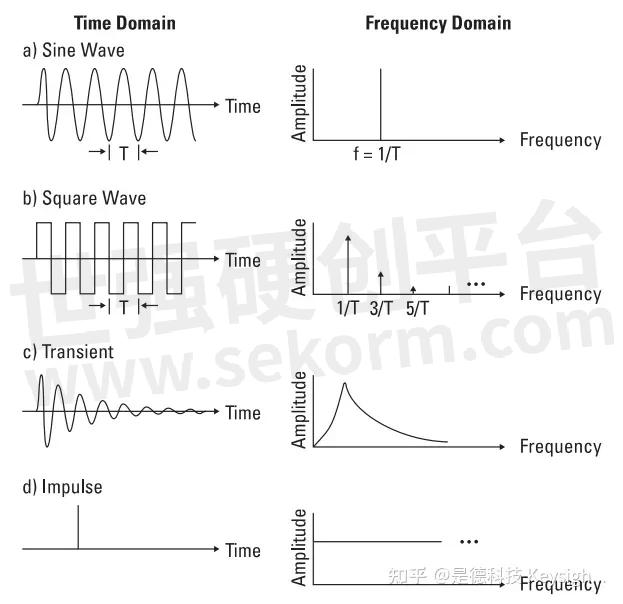
We won't go into the details of the mathematics here, since there are numerous books which cover the theory extensively (see references). Some typical signals represented in the time domain and the frequency domain are shown in Figure 2.

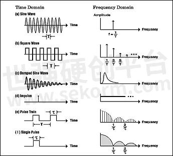
Figure 2: Frequency spectrum examplesThe Fast Fourier Transform

The discrete (or digitized) version of the Fourier transform is called the Discrete Fourier Transform (DFT). This transform takes digitized time domain data and computes the frequency domain representation. While normal Fourier theory is useful for understanding how the time and frequency domain relate, the DFT allows us to compute the frequency domain representation of real-world time domain signals. This brings the power of Fourier theory out of the world of mathematical analysis and into the realm of practical measurements. The Keysight 54600 scope with Measurement/Storage Module uses a particular algorithm, called the Fast Fourier Transform (FFT), for computing the DFT. The FFT and DFT produce the same result and the feature is commonly referred to as simply the FFT.

示波器的快速傅立叶变换（FFT）功能应用 - 示波器的 快速傅里叶变换FFT功能可以快速突出显示电源上耦合信号的频率分布。反之，此类测量又有助于找出噪声信号的源头。这是非常重要的，因为除非发现并解决了这个问题，否则这些信号可能在设计的其他部分转化为噪声，缩减信号裕量，并可能阻碍设计完成原型验证。

The Keysight 54600 series scopes normally digitize the time domain waveform and store it as a 4000 point record. The FFT function uses 1000 of these points (every fourth point) to produce a 500 point frequency domain display. This frequency domain display extends in frequency from 0 to feff /2, where feff is the effective sample rate of the time record (Figure 3a).

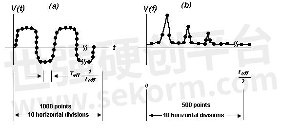
Figure 3

(a) The sampled time domain waveform.

(b) The resulting frequency domain plot using the FFT.

The effective sample rate is the reciprocal of the time between samples and depends on the time/div setting of the scope. For the Keysight 54600 series, the effective sample rate is given by:

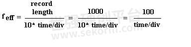
So for any particular time/div setting, the FFT produces a frequency domain representation that extends from 0 to feff/2 (Figure 3b). When the FFT function is active, the effective sample rate is displayed when the time/div knob is turned or the ± key is pressed. Note that the effective sample rate for the FFT can be much higher than the maximum sample rate of the scope. The maximum sample rate of the scope is 20MHz, but the random-repetitive sampling technique places samples so precisely in time that the sample rate seen by the FFT can be as high as 20GHz.

The default frequency domain display covers the normal frequency range of 0 to feff/2. The Center Frequency and Frequency Span controls can be used to zoom in on narrower frequency spans within the basic 0 to feff/2 range of the FFT. These controls do not affect the FFT computation, but instead cause the frequency domain points to be replotted in expanded form.

Aliasing

The frequency feff/2 is also known as the folding frequency. Frequencies that would normally appear above feff/2 (and, therefore, outside the useful range of the FFT) are folded back into the frequency domain display. These unwanted frequency components are called aliases, since they erroneously appear under the alias of another frequency. Aliasing is avoided if the effective sample rate is greater than twice the bandwidth of the signal being measured.

The frequency content of a triangle wave includes the fundamental frequency and a large number of odd harmonics with each harmonic smaller in amplitude than the previous one. In Figure 4a, a 26kHz triangle wave is shown in the time domain and the frequency domain. Figure 4b shows only the frequency domain representation. The leftmost large spectral line is the fundamental. The next significant spectral line is the third harmonic. The next significant spectral line is the fifth harmonic and so forth. Note that the higher harmonics are small in amplitude with the 17th harmonic just visible above the FFT noise floor. The frequency of the 17th harmonic is 17 x 26kHz = 442kHz, which is within the folding frequency of feff /2, (500kSa/sec) in Figure 4b. Therefore, no significant aliasing is occurring.

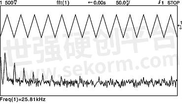
Figure 4a: The time domain and frequency domain displays of a 26kHz triangle wave.

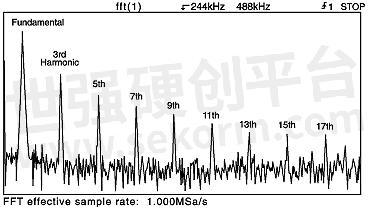
Figure 4b: Frequency spectrum of a triangle wave.

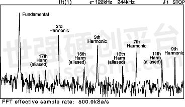
Figure 4c: With a lower effective sample rate, the upper harmonics appear as aliases.

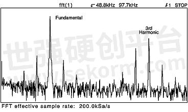
Figure 4d: With an even lower effective sample rate, only the fundamental and third harmonic are not aliased.

Figure 4c shows the FFT of the same waveform with the time/div control turned one click to the left, resulting in an effective sample rate of 500kSa/sec and a folding frequency of 250kSa/sec. Now the upper harmonics of the triangle wave exceed the folding frequency and appear as aliases in the display. Figure 4d shows the FFT of the same triangle wave, but with an even lower effective sample rate (200kSa/sec) and folding frequency (100kSa/sec). This frequency plot is severely aliased.

Often the effects of aliasing are obvious, especially if the user has some idea as to the frequency content of the signal. Spectral lines may appear in places where no frequency components exist. A more subtle effect of aliasing occurs when low level aliased frequencies appear near the noise floor of the measurement. In this case the baseline can bounce around from acquisition to acquisition as the aliases fall slightly differently in the frequency domain.

Aliased frequency components can be misleading and are undesirable in a measurement. Signals that are bandlimited (that is, have no frequency components above a certain frequency) can be viewed alias-free by making sure that the effective sample rate is high enough. The effective sample rate is kept as high as possible by choosing a fast time/div setting. While fast time/div settings produce high effective sample rates, they also cause the frequency resolution of the FFT display to degrade.

If a signal is not inherently bandlimited, a lowpass filter can be applied to the signal to limit its frequency content (Figure 5). This is especially appropriate in situations where the same type of signal is measured often and a special, dedicated lowpass filter can be kept with the scope.

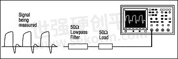
Figure 5: A lowpass filter can be used to band limit the signal, avoiding aliasing.

Leakage*

The FFT operates on a finite length time record in an attempt to estimate the Fourier Transform, which integrates over all time. The FFT operates on the finite length time record, but has the effect of replicating the finite length time record over all time (Figure 6). With the waveform shown in Figure 6a, the finite length time record represents the actual waveform quite well, so the FFT result will approximate the Fourier integral very well.

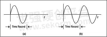
Figure 6

(a) A waveform that exactly fits one time record.

(b) When replicated, no transients are introduced.

However, the shape and phase of a waveform may be such that a transient is introduced when the waveform is replicated for all time, as shown in Figure 7. In this case, the FFT spectrum is not a good approximation for the Fourier Transform.

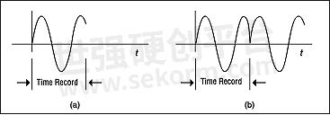
Figure 7

(a) A waveform that does not exactly fit into one time record.

(b) When replicated, severe transients are introduced, causing leakage in the frequency domain.

Since the scope user often does not have control over how the waveform fits into the time record, in general, it must be assumed that a discontinuity may exist. This effect, known as LEAKAGE, is very apparent in the frequency domain. The transient causes the spectral line (which should appear thin and slender) to spread out as shown in Figure 8.

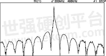
Figure 8 Leakage occurs when the normally thin spectral line spreads out in the frequency domain.

The solution to the problem of leakage is to force the waveform to zero at the ends of the time record so that no transient will exist when the time record is replicated. This is accomplished by multiplying the time record by a WINDOW function. Of course, the window modifies the time record and will produce its own effect in the frequency domain. For a properly designed window, the effect in the frequency domain is a vast improvement over using no window at all.1 Four window functions are available in the Keysight 54600 scopes: Hanning, Flattop, Rectangular and Exponential.

The Hanning window provides a smooth transition to zero as either end of the time record is approached. Figure 9a shows a sinusoid in the time domain while Figure 9b shows the Hanning window which will be applied to the time domain data. The windowed time domain record is shown in Figure 9c. Even though the overall shape of the time domain signal has changed, the frequency content remains basically the same. The spectral line associated with the sinusoid spreads out a small amount in the frequency domain as shown in Figure 10.2 (Figure 10 is expanded in the frequency axis to show clearly the shape of the window in the frequency domain.)

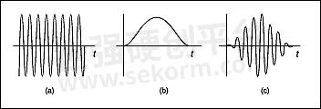
Figure 9

(a) The original time record.

(b) The Hanning Window.

(c) The windowed time record.

The shape of a window is a compromise between amplitude accuracy and frequency resolution. The Hanning window, compared to other common windows, provides good frequency resolution at the expense of somewhat less amplitude accuracy.

The FLATTOP window has fatter (and flatter) characteristic in the frequency domain, as shown in Figure 11. (Again, the figure is expanded in the frequency axis to show clearly the effect of the window.) The flatter top on the spectral line in the frequency domain produces improved amplitude accuracy, but at the expense of poorer frequency resolution (when compared with the Hanning window).

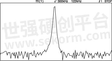
Figure 10 The Hanning Window has a relatively narrow shape in the frequency domain.

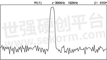
Fig. 11: The flattop window has a wider, flat-topped shape in the frequency domain.

The Rectangular window (also referred to as the Uniform window) is really no window at all; all of the samples are left unchanged. Although the uniform window has the potential for severe leakage problems, in some cases the waveform in the time record has the same value at both ends of the record, thereby eliminating the transient introduced by the FFT. Such waveforms are called SELF-WINDOWING. Waveforms such as sine bursts, impulses and decaying sinusoids can all be self-windowing.

A typical transient response is shown in Figure 12a. As shown, the waveform is self-windowing because it dies out within the length of the time record, reducing the leakage problem.

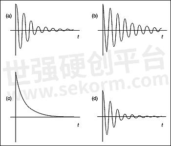
Figure 12

(a) A transient response that is self-windowing.

(b) A transient response which requires windowing.

(c) The exponential window.

(d) The windowed transient response.

If the waveform does not dissipate within the time record (as shown in Figure 12b), then some form of window should be used. If a window such as the Hanning window were applied to this waveform, the beginning portion of the time record would be forced to zero. This is precisely where most of the transient's energy is, so such a window would be inappropriate.

A window with a decaying exponential response is useful in such a situation. The beginning portion of the waveform is not disturbed, but the end of the time record is forced to zero. There still may be a transient at the beginning of the time record, but this transient is not introduced by the FFT. It is, in fact, the transient being measured. Figure 12c shows the exponential window and Figure 12d shows the resulting time domain function when the exponential window is applied to Figure 12b. The exponential window is inappropriate for measuring anything but transient waveforms.

1The effect of a time domain window in the frequency domain is analogous to the shape of the resolution bandwidth filter in a swept spectrum analyzer.

2The shape of a perfect sinusoid in the frequency domain with a window function applied is the Fourier transform of the window function.

Selecting a Window

Most measurements will require the use of a window such as the Hanning or Flattop windows. These are the appropriate windows for typical spectrum analysis measurements. Choosing between these two windows involves a tradeoff between frequency resolution and amplitude accuracy. Having used the time domain to explain why leakage occurs, now the user should switch into frequency domain thinking. The narrower the passband of the window's frequency domain filter, the better the analyzer can discern between two closely spaced spectral lines. At the same time, the amplitude of the spectral line will be less certain. Conversely, the wider and flatter the window's frequency domain filter is, the more accurate the amplitude measurement will be and, of course, the frequency resolution will be reduced. Choosing between two such window functions is really just choosing the filter shape in the frequency domain.

The rectangular and exponential windows should be considered windows for special situations. The rectangular window is used where it can be guaranteed that there will be no leakage effects. The exponential window is for use when the input signal is a transient.3

A Matter of Perspective

In this chapter we introduce the concepts of the time, frequency and modal domains. These three ways of looking at a problem are interchangeable; that is, no information is lost in changing from one domain to another. The advantage in introducing these three domains is that of a change of perspective. By changing perspective from the time domain, the solution to difficult problems can often become quite clear in the frequency or modal domains.  After developing the concepts of each  domain, we will introduce the types of instrumentation available. The merits of each generic instrument type are discussed to give the reader an appreciation of the advantages and disadvantages of each approach.

The Time Domain

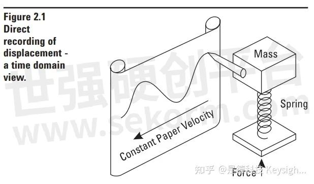
The traditional way of observing signals is to view them in the time domain. The time domain is a record of what happened to a parameter of the system versus time. For instance, Figure 2.1 shows a simple spring mass system where we have attached a pen to the mass and pulled a piece of paper past the pen at a Constant rate. The resulting graph is a record of the displacement of the mass versus time, a time do main view of displacement.  Such direct recording schemes are sometimes used, but it usually is much more practical to convert the parameter of interest to an electrical signal using a transducer.  Transducers are commonly available to change a wide variety of parameters to electrical signals. Microphones, accelerometers, load cells, conductivity and pressure probes are just a few examples.

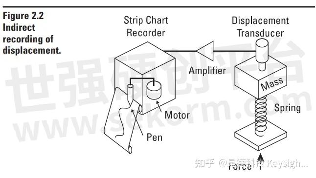
This electrical signal, which represents a parameter of the system, can be recorded on a strip chart recorder as in Figure 2.2. We can adjust the gain of the system to calibrate our measurement. Then we can reproduce exactly the results of our simple direct recording system in Figure 2.1.  Why should we use this indirect approach? One reason is that we are not always measuring dis placement.  We then must convert the desired parameter to the displacement of the recorder pen. Usually, the easiest way to do this is through the intermediary of electronics. However, even when measuring displacement, we would normally use an indirect approach.  Why? Primarily because the system in Figure 2.1 is hopelessly ideal. The mass must be large enough and the spring stiff enough so that the pens mass and drag on the paper will not affect the results appreciably. Also, the deflection of the mass must be large enough to give a usable result, otherwise a mechanical lever system to amplify the motion would have to be add ed with its attendant mass and friction.   With the indirect system a transducer can usually be selected which will not significantly affect the measurement.  This can go to the extreme of commercially available displacement transducers which do not even contact the mass. The pen deflection can be easily set to any desired value by controlling the gain of the electronic amplifiers.

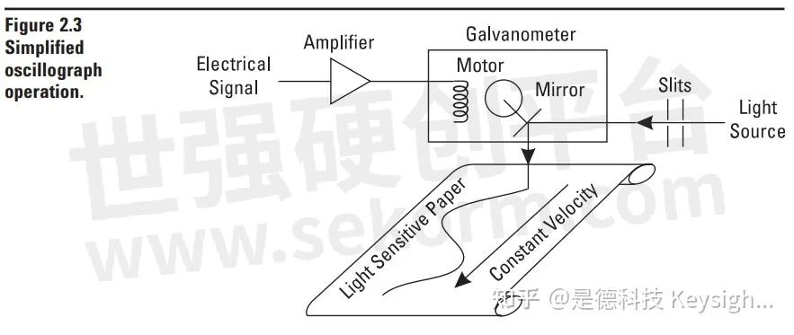
This indirect system works well until our measured parameter begins to change rapidly. Because of the mass of the pen and record er mechanism and the power limitations of its drive, the pen can only move at finite velocity. If the measured parameter changes faster, the output of the recorder will be in error. A common way to re duce this problem is to eliminate the pen and record on a pho to sensitive paper by deflecting a light beam. Such a device is called an oscillograph. Since it is only necessary to move a small, light-weight mirror through a very small angle, the oscillograph can respond much faster than a strip chart recorder.

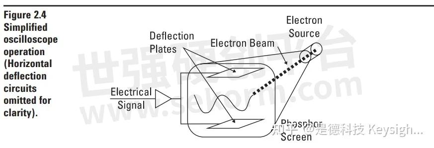
Another common device for displaying signals in the time domain is the oscilloscope. Here an electron beam is moved using electric fields. The electron beam is made visible by a screen of phosphorescent material.   It is capable of accurately displaying signals that vary even more rapidly than the oscillograph can handle.  This is because it is only necessary to move an electron beam, not a mirror.

The strip chart, oscillograph and oscilloscope all show displacement versus time. We say that changes in this displacement rep re sent the variation of some parameter versus time. We will now look at another way of representing the variation of a pa ram e ter.

The Frequency Domain

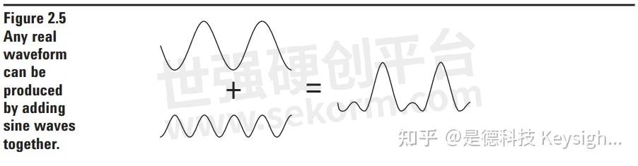
It was shown over one hundred years ago by Baron Jean Baptiste Fourier that any waveform that exists in the real world can be generated by adding up sine waves. We have illustrated this in Figure 2.5 for a simple waveform composed of two sine waves.  By picking the amplitudes, frequencies and phases of these sine waves correctly, we can generate a waveform identical to our desired signal.  Conversely, we can break down our real-world signal into these same sine waves. It can be shown that this combination of sine waves is unique; any real-world signal can be represented by only one combination of sine waves.  Figure 2.6a is a three-dimensional graph of this addition of sine waves.  Two of the axes are time and amplitude, familiar from the time domain.  The third axis is frequency which allows us to visually separate the sine waves which add to give us our complex waveform. If we view this three-dimensional graph along the frequency axis, we get the view in Figure 2.6b. This is the time do main view of the sine waves. Adding them together at each instant of time gives the original wave form.

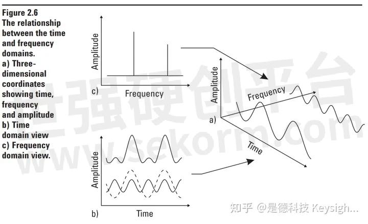
However, if we view our graph along the time axis as in Figure 2.6c, we get a totally different picture. Here we have axes of amplitude versus frequency, what is commonly called the frequency domain. Every sine wave we separated from the input appears as a vertical line. Its height represents its amplitude, and its position represents its frequency. Since we know that each line represents a sine wave, we have uniquely characterized our input signal in the frequency domain*. This frequency domain representation of our signal is called the spectrum of the signal.  Each sine wave line of the spectrum is called a component of the total signal.

Understanding Dynamic Signal Analysis

We saw in the previous chapter that the Dynamic Signal Analyzer has the speed advantages of par Alle filter analyzers without their low-resolution limitations. In addition, it is the only type of analyzer that works in all three domains. In this chapter we will de vel op a fuller understanding of this important analyzer family, Dynamic Signal Analyzers. We begin by presenting the properties of the Fast Fourier Transform (FFT) upon which Dynamic Signal Analyzers are based.  No proof of these properties is given, but heuristic arguments as to their validity are used where appropriate.  We then show how these FFT properties cause some un de sir able characteristics in spectrum analysis like aliasing and leakage. Having demonstrated a potential difficulty with the FFT, we then show what solutions are used to make practical Dynamic Signal Analyzers. Developing this basic knowledge of FFT characteristics makes it simple to get good results with a Dynamic Signal Analyzer in a wide range of measurement problems.

Section 1: FFT Properties  

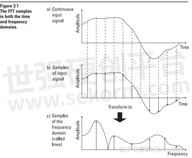
FFT is an algorithm* for transforming data from the time domain to the frequency domain. Since this is exactly what we want a spectrum analyzer to do, it would seem easy to implement a Dynamic Signal Analyzer based on the FFT. However, we will see that there are many factors which complicate this seemingly straightforward task.  First, because of the many calculations involved in transforming domains, the transform must be implemented on a digital com put er if the results are to be sufficiently accurate. Fortunately, with the advent of microprocessors, it is easy and inexpensive to incorporate all the needed computing power in a small instrument package. Note, however, that we cannot now transform to the frequency domain in a continuous manner, but instead must sample and digitize the time domain input. This means that our algorithm transforms digitized samples from the time domain to samples in the frequency domain as shown in Figure 3.1.** Because we have sampled, we no longer have an exact representation in either domain. However, a sampled representation can be as close to ideal as we de sire by placing our samples clos er together. Later in this chapter, we will consider what  sample spacing is necessary to guarantee ac cu rate results.

* An algorithm is any special mathematical method of solving a certain kind of problem, e.g., the technique you use to balance your checkbook. ** To reduce confusion about which domain we are in, samples in the frequency domain are called lines.

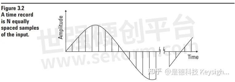
Time Records

A time record is defined to be N consecutive, equally spaced samples of the input. Because it makes our transform algorithm simpler and much faster, N is restricted to be a multiple of 2, for instance 1024.

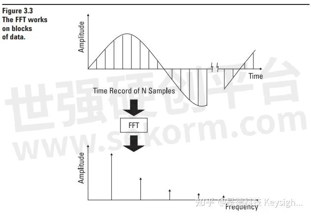
As shown in Figure 3.3, this time record is transformed as a complete block into a complete block of frequency lines. All the samples of the time record are need ed to compute each and every line in the frequency domain. This is in contrast to what one might expect, namely that a single time domain sample transforms to exactly one frequency domain line. Understanding this block processing property of the FFT is crucial to under standing many of the prop er ties of the Dynamic Signal Analyzer.

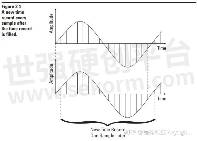
For instance, because the FFT transforms the entire time record block as a total, there cannot be valid frequency domain results until a complete time record has been gathered. However, once completed, the oldest sample could be discarded, all the samples shifted in the time record, and a new sample added to the end of the time record as in Figure 3.4. Thus, once the time record is initially filled, we have a new time record at every time domain sample and therefore could have new valid results in the frequency domain at every time domain sample.  This is very similar to the behavior of the parallel Fi Fast Fourier Transform (FFT) later analyzers described in the previous chap ter. When a signal is first applied to a parallel-filter analyzer, we must wait for the filters to respond, then we can see very rapid changes in the frequency domain.  With a Dynamic Signal Analyzer, we do not get a valid result until a full-time record has been gathered. Then rapid changes in the spectra can be seen.

The relationship between the time and frequency domains.   a) Three dimensional coordinates showing time, frequency and amplitude b) Time domain view c) Frequency domain view.

Frequency spectrum examples

Time Domain and Frequency Domain Measurements in 89600 VSA Software

Measurements made in the time domain are the basis of all measurements in the 89600 VSA software. The time domain display shows a parameter (usually amplitude) versus time. You are probably familiar with time domain measurements as they appear in an oscilloscope. Similar measurements may be viewed with the time measurement data capability.

"PathWave 89600 VSA软件能够执行矢量信号分析，利用信号在时域、频谱域和调制域中的迹线来显示信号质量。 与频谱分析仪、信号分析仪、网络分析仪等仪器兼容。"

Frequency-domain displays show a parameter (again, usually amplitude) versus frequency. A spectrum analyzer takes an analog input signal—a time-domain signal—and uses the Fast Fourier Transform (FFT) to convert it to the frequency domain. The resulting spectrum measurement shows the energy of each frequency component at each point along the frequency spectrum.

Many signals not visible in the time domain (such as noise and distortion products) are clearly visible in the frequency domain. Because spectrum displays show frequency components distributed along the frequency axis, it's possible to view many different signals at the same time. This is why the spectrum analyzer is such a useful tool for looking at complex signals—it lets you easily measure (and compare) the frequency and amplitude of individual components.

The Y axis (amplitude)

Time-domain measurements are usually viewed with a linear X axis and a linear Y axis (think of an oscilloscope). Frequency-domain measurements are sometimes viewed with a linear Y axis and a linear X axis, but usually must be viewed with a logarithmic Y axis, because this is the only way to view very small signals and much larger signals simultaneously.

Let's look at the spectrum of a sine wave. Because the amplitude of any harmonic is small relative to the fundamental frequency, it's nearly impossible to view a harmonic on the same display as the fundamental unless the Y-axis scale is logarithmic. That's why most measurements made with spectrum analyzers use a logarithmic amplitude scale—a scale based on decibels. And because the dB scale is by definition logarithmic, there's no need to use logarithmically-spaced graticule lines.

The X axis (frequency)

Sometimes it's convenient to use a logarithmic X axis. Perhaps most familiar to you is the frequency response measurement. This is traditionally displayed with a log X axis (frequency) versus a log Y axis (relative magnitude).

But most measurements do not require a logarithmic frequency scale. In fact, when making spectrum measurements it's easier to characterize harmonics with a linear X-axis scale because harmonics that are multiples of the same fundamental will appear at evenly spaced intervals.